Making a packing spreadsheet
Being the unique person I am, I love traveling. Oftentimes I end up getting deep into trying to optimize my packing methods. There are dozens of tools online designed to help with this exact thing (services like Lighterpack or GearGrams). But, being handy with code, I decided to dabble in the subject on my own.
One of the most important things in packing is the overall weight of the pack, and I always want to know what type of things are the heaviest. I also want to be able to run random queries on my data, whatever it is that I’m trying to learn. I want to have an inventory of items (backpacks, clothes, storage solutions) which I can plug in and out of a spreadsheet to see how the resulting picture changes on the go. Working with software as my day job, I’d also like for the solution to be automated whenever possible.
Google Spreadsheets turned out to be the perfect solution, providing the ability to quickly sum up the weight of my things and output insights about the data.
Final Result
Here’s a link to the spreadsheet, I encourage the reader to copy and play around with in anyway you see fit.
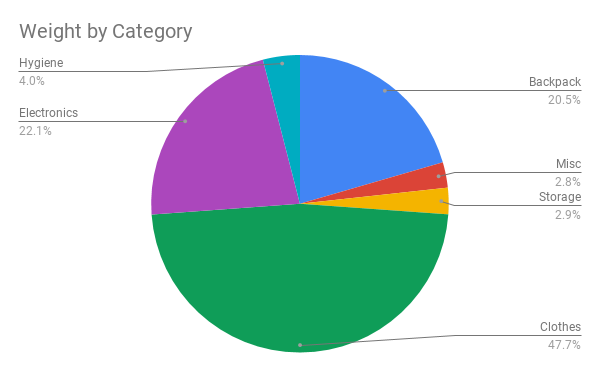
Here’s the final result for a multi-day trip I will have for this year. As you can see, my pack weighs around 3 kilograms or a bit over 6 freedom units (not including water). My recently purchased Nintendo Switch is the heaviest item (and it’s worth every gram as it makes flying tolerable), but clothes take up most of the weight:
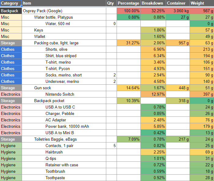
I use indentation levels to show that some items are contained within other items. This also lets me calculate the absolute and relative weights of a whole container with everything inside of it (see fields labeled “Container” and “Percentage”).
The “Weight” and the “Breakdown” fields indicate absolute and relative item weight respectively, which accounts for quantity of the item (quantity defaults to 1 if not explicitly set). Weight-related fields are color coded from lightest items in green to heaviest items in red.
Categories are used to group items and execute queries on the data and learn insights like these:
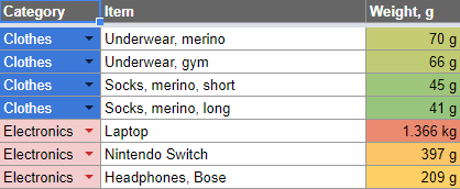
There’s a separate sheet where I enter item names, categories, and weights, which I then use to automatically populate values above and autofill item names in the primary sheet:
The Technical Details
I haven’t worked with Google Spreadsheets (or Excel for that matter) a lot in the past, but with an access to clear documentation (and a hundred of web searches later) it was straightforward to get the hang of the it.
I started off by manually populating the final result sheet, manually adjusting formulas for Container/Percentage cells, as I had no idea how I would detect the indentation yet. I like when things look pretty, so I applied conditional formatting rules right away, and the looks of the sheet really haven’t changed throughout the process.
Next, I created an inventory sheet, which I wanted to use as a source of data in the resulting sheet. A few Google searches and some trial & error resulted in a lookup formula:
=ArrayFormula(
 IF(
   NOT(ISBLANK($B2)),
   INDEX(InventoryCategories, MATCH($B2, InventoryItems, 0)),
   IF(
     NOT(ISBLANK($C2)),
     INDEX(InventoryCategories, MATCH($C2, InventoryItems, 0)),
     INDEX(InventoryCategories, MATCH($D2, InventoryItems, 0))
   )
  )
)
ArrayFormula is necessary in order to create arrays on the fly without printing intermediate results in the spreadsheet. InventoryItems and InventoryCategories are named ranges referring to item names and categories in the inventory sheet. MATCH finds an index of a first occurrence of the item name in the sheet, and retrieves corresponding category name. An item weight is retrieved by the exact same principle.
Trying to find the container weight took a lot more time, and resulted in a lot more headache. Solution for handling indentation in Google Spreadsheets wasn’t as elegant as I would have hoped for, but it got the job done:
=ArrayFormula(
     SUM(
       $I2:INDIRECT(
         CONCATENATE(
           "$I",
           ROW() + IF(
             NOT(ISBLANK($B2)),
             MATCH(FALSE, ISBLANK($B3:$B), 0),
             MATCH(FALSE, ISBLANK($C3:$C), 0)
           ) - 1
         )
       )
     )
The formula above finds the first non-empty cell in a column. It starts searching from the next row (for example, for an item on a second row, we look at the third row and below). After it knows which row first non-empty cell is in, the formula turns it into a string (column $I contains item weights) and use it as an upper bound of a sum of the weights. Finished formula is a bit longer (it adds sugar to only display the number when needed), and if you’re interested - you can look it up in the spreadsheet.
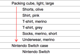
For example, in the screenshot above, the formula will start looking at cells in a column right after the “Packing cube”. As soon as it finds a non-empty cell (“Nintendo Switch case”), the formula will determine this row to be an upper boundary. The formula then will sum weights starting with a “Packing cube” row, and up to but not including “Nintendo Switch case” row.
The rest involved many small tweaks, adding pretty colors, hiding N/A errors and zeroes, and trying to find the perfect shade for column borders.
And, since you made it this far, here’s how the numbers above look in the real world:
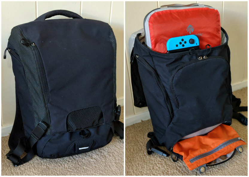
Hopefully you found this useful, or at least somewhat entertaining. There’s a lot of room for improvement, and I aimed to provide a framework and a few basic ideas for building a spreadsheet to accommodate one’s twisted ultralight needs.